Note: This document is for an older version of the Gro API Client. Please see the latest documentation.

Modeling Resources

Gro Crop Cover

Gro’s proprietary high-resolution crop covers are currently used in the Gro yield models. These have proven very successful i.e. more accurate for yield modeling than the best available alternatives. Gro does not plan on developing a yield model for every crop or region in the world, so our models will always be limited to the regions and crops where we can help push the envelope. Users can access our crop covers in the Gro web app and the API, or from the download links below. In the web app and API, users can interact with detailed cropland covers that indicate the intensity of crop cover for a particular pixel. Below users can download .tif files of low and high-confidence crop covers which represent, as a binary value, whether a crop is growing in a specific pixel.

Methodology

Crop covers for past seasons

In order to remove irrelevant data pixels (i.e., pixels that are not representative of the crop in study), we create/derive crop specific covers for each past crop season, as described here (see also Creating a basic customizable framework for crop detection using Landsat imagery. This is necessary for each year, due to crop rotations and other changes in the area where crops are planted. Moreover, even with per-season covers, there is an additional challenge for in-season crop yield forecasting, because the current season crop cover is usually not available until the beginning of the following year.

In-season crop cover

For current season forecasting, since we’re starting well before the growing period, there is no universal approach that provides the best cover. Instead, we use the series of covers for prior seasons to create a few different covers for the current season. Together, these current season covers can be thought of as providing supersets and subsets of the true planted area. The combination of the various covers provides the information needed for yield forecasting purposes.

For any cover, the following current season covers are created:

• a low-confidence version is created by an OR of the years, i.e., choosing pixels that have been the crop in question for at least one year in the history of the cropland data layers. In other words, the low-confidence cover answers the question “was the crop planted here in 2000 or in 2001 or in 2002 …”. This can be thought of as an upper bound of the true area. Or equivalently, for each pixel, a prediction with high recall and low precision.

• a high-confidence cover version is created by an AND of the years, i.e., selecting pixels that have always been the crop in question over the entire history of the prior season covers, so long as that region has been in the data layers. In other words, it answers the question “was the crop planted here in 2000 and in 2001 and in 2002 …” This it can be seen as a lower bound of the true area. Or equivalently, for each pixel, a prediction with low recall and high precision.

Additional refinements:

• a clumped version is obtained by removing clusters with a total number of fewer than 8 pixels.

US Corn

Yearly corn covers (binary) were extracted from USDA NASS Cropland Data Layers (CDL) for the US Corn Belt, which includes 10 states: Illinois, Indiana, Iowa, Kansas, Minnesota, Missouri, Nebraska, Ohio, South Dakota, and Wisconsin, from 1999 to 2015. Note that not all states were covered in the yearly covers prior to 2008 due to growing coverage of NASS CDL from 1999 to 2008.

A low-confidence cover and a high-confidence cover were made from those yearly crop covers. Each of them was further clumped to remove erroneous pixels, which gave us two more static corn covers.

Click the links below to download TIF files of in-season covers:

• low confidence
• high confidence
• low confidence clumped
• low confidence clumped

US Soy

Yearly soy covers were extracted from the NASS CDL the same way as corn, except that the entire contiguous US was included. In this case we end up using only one cover:

We start in 2008, because including years prior to 2008 reduces the accuracy for yield modeling purposes. A high-confidence cover is not used, as it was found to not help the yield modeling accuracy. Both of these observations seem to reflect the fact that, in the US, the areas where soybeans are planted have been changing relatively more than the corn areas, which makes older crop covers less informative in this case.

Click the link below to download TIF files of in-season covers:

• low confidence

Argentina Soy

Argentina does not have an equivalent of the US CDL data, so annual soybean covers had to be created by Gro. These covers were created annually and ranged from 2007-2016 using the following methodology.

The signals for classification of soy in Argentina were from optical sensors from Landsat 5, 7, and 8 along with Sentinel-2. First, a set of false color images were created from the shortwave infrared (SWIR ~1.62µm) band, near infrared (NIR ~0.85µm) band, and visible red (Red ~0.66µm) band. which were temporally classified using the crop calendars in Gro for the primary season of soybean production over the country. These were divided into two images, one taking the median pixel value over the time period that planting occurred and the other taking the median pixel value over the time period when growth occurred. The false color image was created. This was done because studies have shown that SWIR-NIR-Red false color composites accurately discriminate between vegetation, soil, and water due to the spectral properties of the channels.

After this was completed, the false color images were transformed from a normal RGB (Red-Green-Blue) color space into a Hue-Saturation-Value (HSV) color space where the Hue band is subsequently isolated. By isolating the Hue pixel values, we solve the problems resulting from variations in brightness level (owed to the Value) and chromatic modulation (from the Saturation) from pixel to pixel. By doing this the Hue pixel values identified as soil generally range on the low end of pixel values while vegetation accounts for the middle range with water taking up the high end range. By subtracting the vegetation hue layer from the soil hue layer and isolating the top portion of the pixel values (pixels greater than or equal to 0.14), what’s left is an image that highlights areas which were soil during the planting phase and vegetation during the growth phase. Those areas are inclined to only be crops during those specific times during the crop cycle (i.e., forests, grasslands, and pastures tend to not change in sync with the cropland) although it is not yet know what specific crops they are, only that their growth cycle matches that of the crop cycle given in the crop calendars.

Once those unidentifiable crops have been found, a simple ratio was used to identify soy from other crops. For the case of soy, we use a simple ratio of: SWIR/Red values from the growing season, where SWIR represents the shortwave infrared band (~1.62µm) and Red represents the red band in the visible spectrum (~0.66µm). High values of this simple ratio were shown to be very distinctive at identifying soy when validated against the NASS Cropland Data Layers in the US.

A low-confidence cover and a high-confidence cover were made from those yearly crop covers. Each of them were further clumped to remove erroneous pixels, which gave us two more static soy covers.

Click the links below to download TIF files of in-season covers:

• low confidence
• high confidence
• low confidence clumped
• low confidence clumped

India Wheat

Since India does not have the equivalent of NASS CDL available to the public, we use a technique similar to the one used for Argentina. The covers were also classified annually and span years 2007-2017. The methodology was refined slightly in three ways:

• Instead of using a single crop calendar for the entire country, crop calendars specific to individual states were used to create the planting and growth phase images. Subsequently, the corresponding years were mosaicked together before the creation of the confidence covers.

• The simple ratio of SWIR/Red was not used for the identification of wheat. Instead, when comparing images to CDL covers in the US the combination that most closely identified with wheat was the high end of Hue*NDVI*NDWI during the growth phase.

• The final change that was made was the addition of eliminating pixels that were on a slope that was greater than 10°.

A low-confidence cover and a high-confidence cover were made from those yearly crop covers. Each of them were further clumped to remove erroneous pixels, which gave us two more static wheat covers.

Click the links below to download TIF files of in-season covers:

• low confidence
• high confidence
• low confidence clumped
• low confidence clumped

Gro Yield Model Backtest Data

Gro yield models provide live forecasts for crops in different regions around the world. To supplement our in-depth papers on the models, we provide backtesting data for model evaluation and comparisons.

File Formats

For each crop-region pair for which we have a yield model, we provide two csv files for each day in the crop season.

1. national level backtest:

   • file name is of the following format: {DATE}_backtesting_national_{CROP}_{REGION}.csv

   • columns in the file are:

     • year: market year of the backtested prediction

     • pred: yield prediction at the country level of that year

     • unit_id: unit_id that the prediction is in. You can look up the unit by using client.lookup('units', input_unit_id) function.

2. regional level backtest

   • granularity varies among models

   • file name is of the following format: {DATE}_backtesting_{CROP}_{REGION}.csv

   • columns in the file are:

     • year: market year of the backtested prediction

     • region_id: Gro region id that this prediction is for. You can look up the region by using client.lookup('regions', region_id) function.

     • pred: yield prediction of that region in that year

     • unit_id: Gro unit id that the prediction is in. You can look up the unit by using client.lookup('units', input_unit_id) function

Download the Data by Model

Models

Listed below are Gro’s existing models. Each available link will download backtest data (daily frequency) for a whole crop season.

• US Corn
• US Soybeans
• Argentina Soybeans
• Brazil Soybeans
• India Wheat
• Ukraine Wheat
• Russia Wheat (Beta)
• US Hard Red Winter Wheat
• Canada Spring Wheat

NOTE: Our “beta” models have run for less than one full season. At this stage, each model has been fully backtested at monthly frequency across a whole crop season. However, the beta models are still under active development, so the inputs and parameters to the models might change during the current season.

Radio Frequency Interference Effects On SMOS

The attached document details the effect that Radio Frequency Interference (RFI) has on the soil moisture source SMOS: radio-frequency-interference-smos.pdf

TRMM and GPM spatial extents

Spatial extent for geospatial sources is the geographic region that is covered by that source. For the rainfall sources in Gro, it is important to know that the spatial extent is limited by their sources due to coverage limitations of the satellite platforms.

For TRMM (3B42RT), the spatial extent of the data is 50° north to 50° south (red bounding box below) due to the satellite’s coverage and the mission’s focus on tropical regions. While for GPM (3IMERGDL), the spatial extent of the data is 90° north to 90° south, however the “complete” version of the data only extends from 60° north to 60° south (blue bounding box below). This is because the “complete” version masks out observed passive microwave estimates over snowy/icy surfaces, so outside the latitude in the blue bounding box, where IR estimates are not available, precipitation estimates over non-snowy/icy surfaces are recorded as missing (1). This means that while Gro uses the 90° north to 90° south dataset, periodically data outside the 60° north to 60° south bounding box will not be reported.

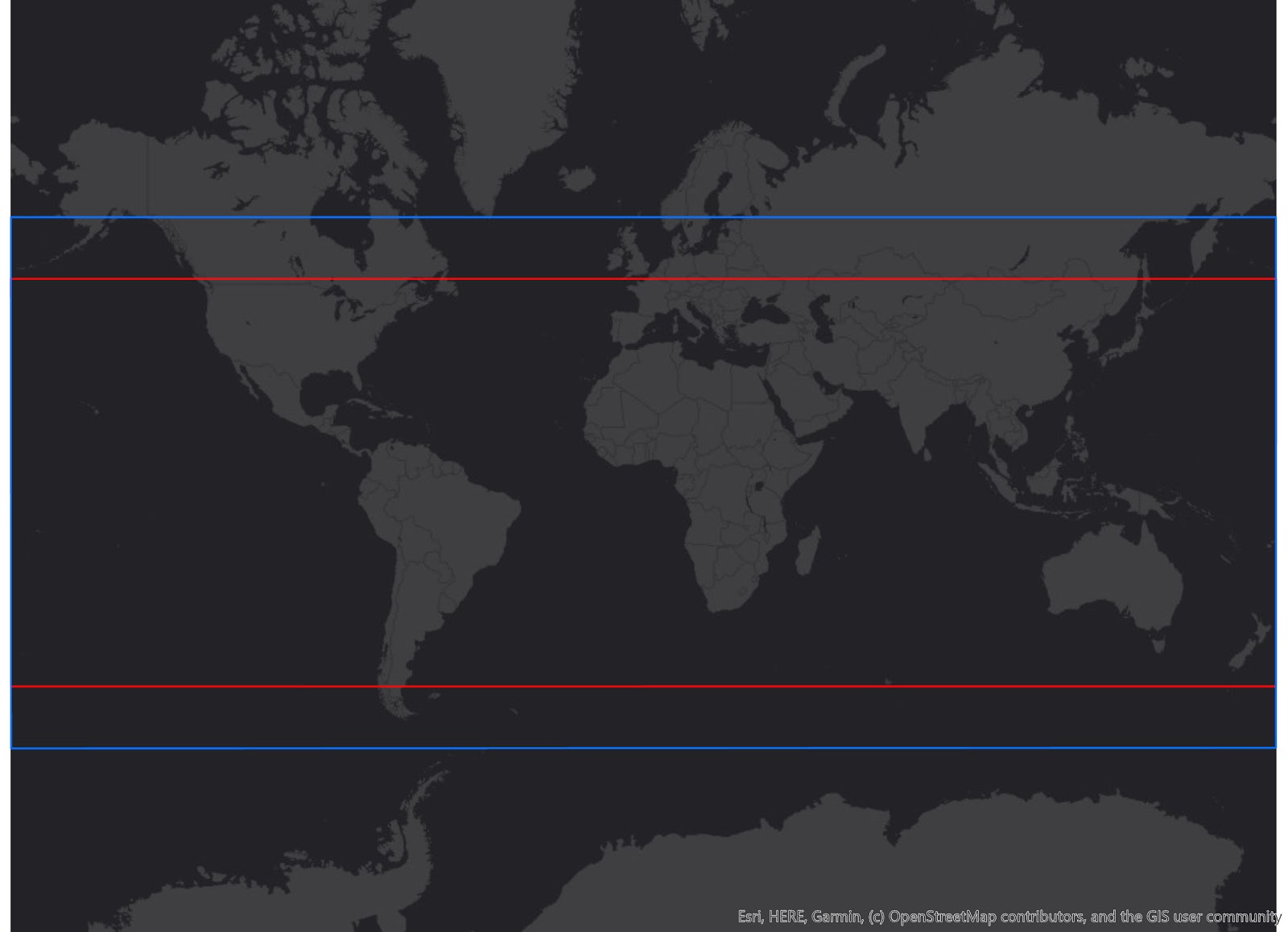
1. Huffman, G. J., Bolvin, D. T., & Nelkin, E. J. (2015). Integrated Multi-satellite Retrievals for GPM (IMERG) technical documentation. NASA/GSFC Code, 612(47), 2019.

Computing Mean Values Amid LST Data Gaps

As an example, the Figure 1 map below, modeled using MODIS sensor data from the Terra satellite, shows India during a monsoon. The monsoon’s path, generally from the southeast to the northwest, can be seen by the level of cloud cover.

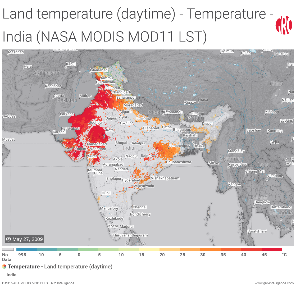
Figure 1. Example of high cloud cover (shown as no data in light grey) during a monsoon in India

Gaps in data caused by cloud coverage can cause daily regional aggregated means to also report no data. Gro requires at least 6% of the pixels in a region to have data for an aggregated mean to be reported. Coverage at less than this percentage can cause outlier values, with aggregated means possibly reporting values more than 10 degrees Celsius higher or lower than what would be measured without cloud coverage.

At times, cloud coverage causes gaps that can occur for multiple days in a row (Figure 2).

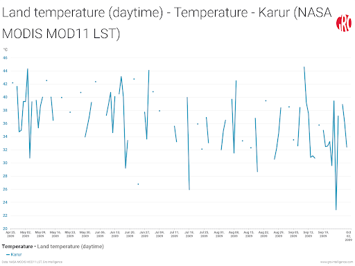
Figure 2. Example of high cloud cover causing missing data points in line charts for a region in India.

Averaging the daily data to longer time steps, such as weekly, smooths the daily variations and allows for easier comparisons of changes over time. But because temperatures can greatly fluctuate from one day to the next, there must be a minimum number of days with data to help minimize the effects of outliers. For land surface temperature data, a minimum of three days with data must be present in order to compute weekly means (Figure 3).

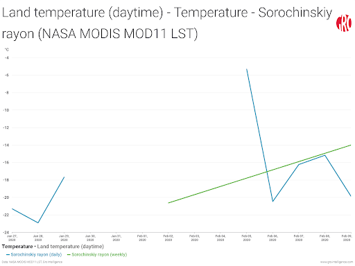
Figure 3. Example of how three days of data (Jan 27-30) will result in a weekly average posted for the week of Jan 27-Feb 2, despite four days of data being missing due to cloud cover. The week of Feb 3-9 has five days with data, which results in a weekly average posted, as well.